In the previous article, we have read in-depth about depth in tensors their rank & data type. We have also built a simple computation graph and under tensor basic operation. If you haven't read the article here's the link.

In this tutorial we are going to cover, linear regression and more in-depth about this also we are going to build a house price prediction App.

1. What is Linear Regression?
2. Understand using Example of Linear Regression?
3. Understanding Learning Algorithm
4. Cost Function
5. Gradient Descent
6. Predicting house price using Tensorflow
7. Cost and the Optimization function

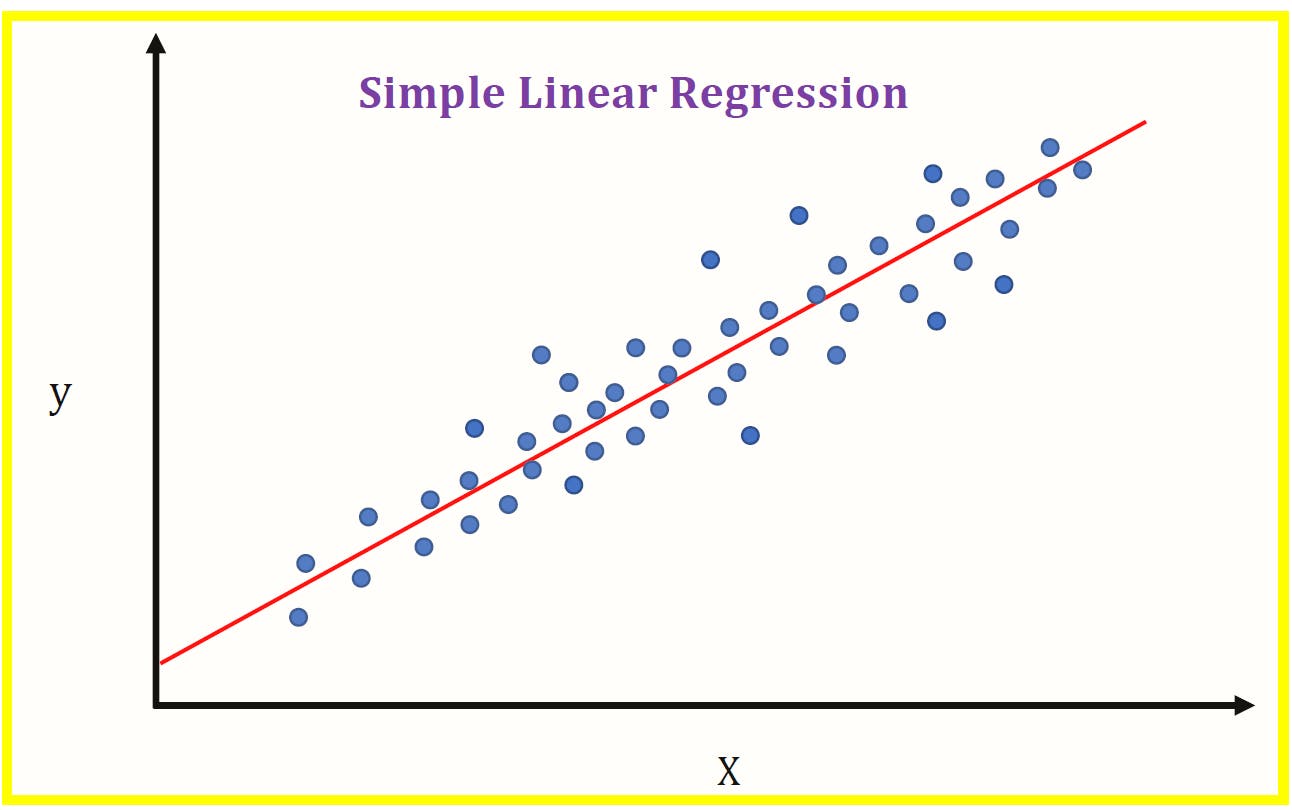
What is Linear Regression?

Linear regression is used for finding the linear relationship between target and one or more predictors.

In another word:

Linear Regression is a Linear Model. This means we will establish a linear relationship between the input variables(X) and single output variable(Y). When the input(X) is a single variable this model is called Simple Linear Regression and when there are multiple input variables(X), it is called Multiple Linear Regression.

Understand using Example

Let's see a simple example of linear regression and how it works in TensorFlow. Here, we solve a simple equation [y=m*x+b]. We will calculate the slope(m) and the intercept(b) of the line that best fits our data.

The following are the steps to calculate the values of m and b.

Step 1. Setting Artificial Data for Regression

Below is the code to create random test data that is linearly separated:

import numpy as np

x_data = np.linspace(0, 10, 10) + np.random.uniform(-1.5, 1.5, 10)
array([-0.69756846  2.24332136  0.87019185  2.91653533  4.87247308  6.14932119
6.61805361  8.68002133  9.38586681  8.80601073])

y_label = np.linspace(0, 10, 10) + np.random.uniform(-1.5, 1.5, 10)
array([-0.39423666  0.68045758  1.83709626  3.82504931  3.74358699  4.82393256
  8.15763383  8.28064161  9.81634308 10.71215334])

Here, we generate ten evenly spaced numbers between 0 and 10 and another ten random values between -1.5 and 1.5. Then, we add these values.

Step 2. Plot the data

If we plot the above data, this is how it would look:

import matplotlib.pyplot as plt
plt.plot(x_data, y_label, '*')

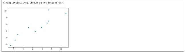
Now, we want to find the best fit (equation of a line) for the given data points.

Step 3. Assign the Variables

Now we're going to assign the TensorFlow variable using tf.Variable().

np.random.rand(2)
array([0.34873631 0.88758771])
# We will use upper random value in m,b

m = tf.Variable(0.34)
b = tf.Variable(0.88)

Here, we have assigned variables m and b randomly using a Numpy random function.

Step 4. Apply Cost Function

The cost function is basically the error between the actual value and the calculated value. We'll read more in-depth later in the tutorial.

Let's find out the cost function:

error = 0

for x,y in zip(x_data, y_label):
    y_hat = m*x + b
    # Our predicted value
    error += (y - y_hat)**2
    # The cost we want to minimize 
    # We'll need to use optimization function the minimization

Step 5. Apply Optimization Function

For training purposes, you need to use an optimizer.

1. Apply the Optimization Function

import tensorflow.compat.v1 as tf
tf.disable_v2_behavior()

optimizer = tf.train.GradientDescentOptimizer(learning_rate=0.001)
train = optimizer.minimize(error)

2. Initialize the variables

init = tf.global_variables_initializer()

3. Create the session and run the computation

with tf.Session() as sess:
    sess.run(init)

    epochs = 100

    for i in range(epochs):

        sess.run(train)

    # Fetch back results
    final_scope, final_intercept = sess.run([m, b])

print(final_scope)
print(final_intercept)

# Output
1.0795033
0.43419915

In this case, it is a gradient descent optimizer, and we need to specify the learning rate.

6. Evaluate the Results

The last step is used to plot the model, i.e., the best-fit line. You can use the plot method to plot the best-fit line.

x_test = np.linspace(-1, 11, 10)
y_pred_plot = final_scope * x_test + final_intercept

plt.plot(x_test, y_pred_plot, 'r')
plt.plot(x_data, y_label, '*')

Full source code here ->

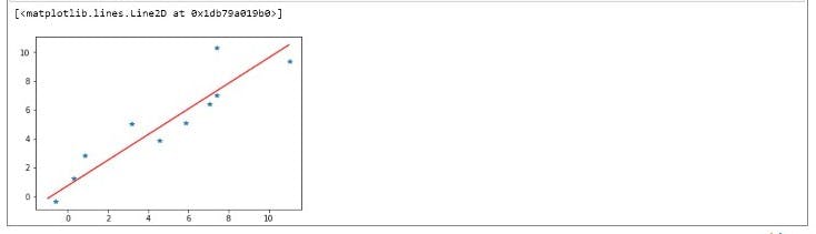
You can see that the line of best fit is passing in between all the data points. If you consider any specific location and calculate the error, it is minimal. This is how you evaluate the results.

Understanding Learning Algorithm

Broadly, there are 3 types of Machine Learning Algorithms

• Supervised Learning: This algorithm consists of a target/outcome variable (or dependent variable) which is to be predicted from a given set of predictors (independent variables). Decision Tree, Regression, Random Forest,
• Unsupervised Learning: In this algorithm, we do not have any target or outcome variable to predict / estimate. Apriori Algorithm, K-means
• Reinforcement Learning: Using this algorithm, the machine is trained to make specific decisions. It works this way: the machine is exposed to an environment where it trains itself continually using trial and error. Markov Decision Process

List of Common Algorithms used in industry:

1. Linear Regression
2. Decision Tree
3. Support Vector Machine (SVM)
4. Naive Bayes
5. KNN
6. K-Means
7. Random Forest
8. Gradient Boosting Algorithms

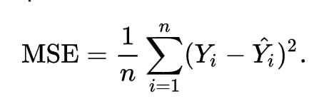
Cost Function

One common function that is often used is mean squared error, which measures the difference between the actual value from the dataset and the estimated value (the prediction).

We can adjust the equation a little to make the calculation a little more simple.

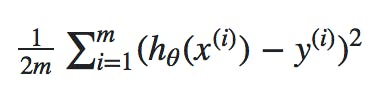
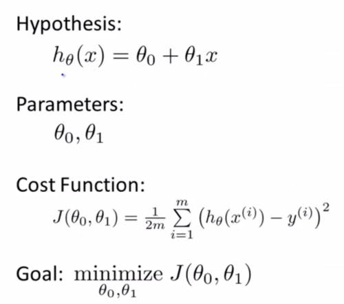
Here is the summary,

• The hypothesis h(x) defines the linear model with parameters θo and θ1.
• The cost function quantifies how good the parameters are. Poor prediction leads to a high value of cost function.

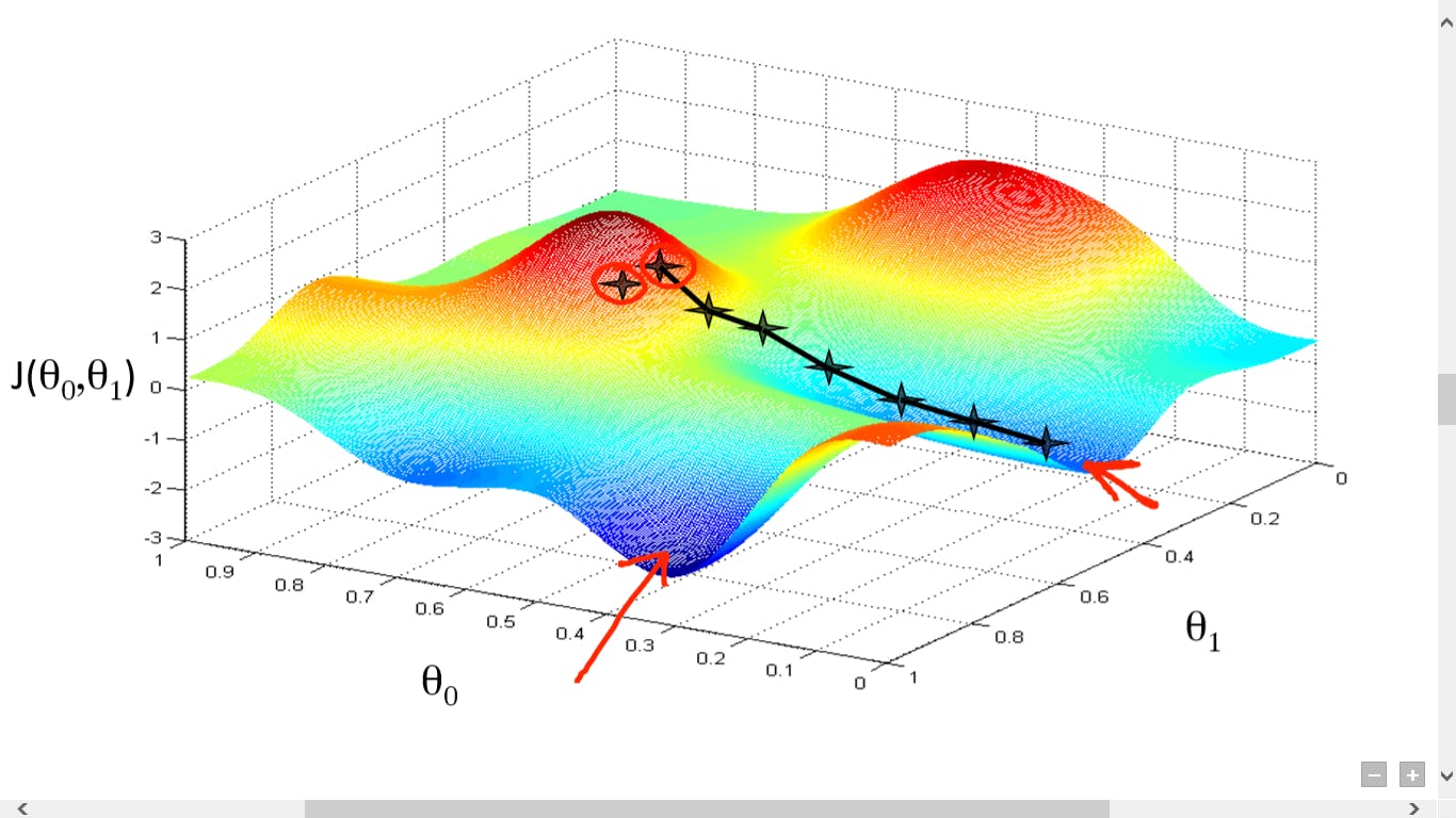
Gradient Descent

Gradient descent is an optimization algorithm used to find the values of parameters (coefficients) of a function (f) that minimizes a cost function (cost).

Gradient descent is best used when the parameters cannot be calculated analytically (e.g. using linear algebra) and must be searched for by an optimization algorithm.

Predicting House Price using Tensorflow

Data Source: github/officialvoltry/.../day_3_housing.csv

California Housing Prices

The data contains information from the 1990 California census. The columns are as follows:

• longitude
• latitude
• housingMedianAge
• totalRooms
• totalBedrooms
• population
• households
• medianIncome
• oceanProximity

Let's get started by importing Libraries (Recommend to use Jupyter )

You can full source code here ->

1. Import Libraries

   import pandas as pd
   import numpy as np
   import matplotlib.pyplot as plt
   import seaborn as sns
   %matplotlib inline
   

2. Load the dataset

   df=pd.read_csv(“housing.csv”)
   df.head()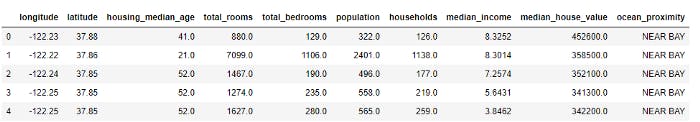
   

   

3. Data Analysis

   df.info()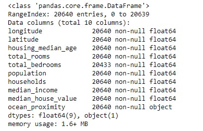
   

   

4. Scaling and Train Test Split

   X = df.drop(‘median_house_value’,axis=1)
   y = df[‘median_house_value’]
   from sklearn.model_selection import train_test_split
   X_train, X_test, y_train, y_test = train_test_split(X,y,test_size=0.3,random_state=42)
   

5. Scaling

   from sklearn.preprocessing import MinMaxScaler
   scaler = MinMaxScaler()
   X_train= scaler.fit_transform(X_train)
   X_test = scaler.transform(X_test)
   

6. Creating a Model

from tensorflow.keras.models import Sequential
from tensorflow.keras.layers import Dense
from tensorflow.keras.optimizers import Adam
from tensorflow.keras.layers import Dropout

model = Sequential()
model.add(Dense(8,activation='relu'))

model.add(Dropout(0.5))
model.add(Dense(3,activation='relu'))

model.add(Dropout(0.5))
model.add(Dense(1))

model.compile(optimizer='adam', loss='mse')

1. Training the Model

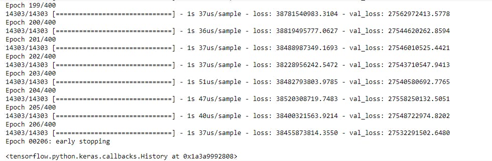
   from tensorflow.keras.callbacks import EarlyStopping
   early_stop = EarlyStopping(monitor='val_loss', mode='min', verbose=1, patience=10)
   model.fit(x=X_train,y=y_train.values,
          validation_data=(X_test,y_test.values),
          batch_size=128,epochs=400, callbacks=[early_stop])
   

1. Plotting graph

   losses = pd.DataFrame(model.history.history)
   losses.plot()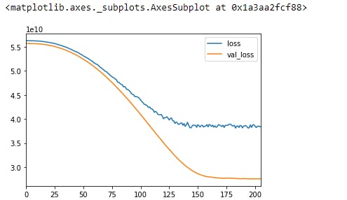
   

   

2. Evaluation

from sklearn.metrics import mean_squared_error,mean_absolute_error
predictions = model.predict(X_test)

mean_absolute_error(y_test,predictions)
# 125709.1601435053

np.sqrt(mean_squared_error(y_test,predictions))
# 165928.57353834526

Next: In the next tutorial, we will read Recurrent Neural Network(RNN)