


In the previous section, we have seen what is machine learning and a basic example of how machine learning works with the super simple example of how our brain works and we have seen the differences between Traditional Development vs Machine Learning.
As I told you earlier, enough let's code and train our first machine learning model.
The Basics
I'll try to keep things simple here, and only introduce the basic concept of TensorFlow. Later in the series will cover more advance and complex problems.
The problem we will solve is to convert from Celsius to Fahrenheit, where the approximate formula is:
f=c×1.8+32
Of course, it would be simple enough to create a conventional Python function that directly performs this calculation, but that wouldn't be machine learning.
Instead, we will give TensorFlow some sample Celsius values (0, 8, 15, 22, 38) and their corresponding Fahrenheit values (32, 46, 59, 72, 100). Then, we will train a model that figures out the above formula through the training process.
Let's Start
Notes: Please create a separate folder and environment for training our machine learning models. You can use `virtualenv or any other environment wrapper.
Import Dependencies
First, import TensorFlow. Here, we're calling it
tffor ease of use. We also tell it to only display errors.Next, import NumPy as
np. Numpy helps us to represent our data as highly performant lists.
import tensorflow as tf
import numpy as np
logger = tf.get_logger()
logger.setLevel(logging.ERROR)
`
Set up training data
As we saw before, supervised Machine Learning is all about figuring out an algorithm given a set of inputs and outputs.
Since the task is to create a model that can give the temperature in Fahrenheit when given the degrees in Celsius, we create two lists celsius_q and fahrenheit_a that we can use to train our model.
celsius_q    = np.array([-40, -10,  0,  8, 15, 22,  38],  dtype=float)
fahrenheit_a = np.array([-40,  14, 32, 46, 59, 72, 100],  dtype=float)

for i,c in enumerate(celsius_q):
  print("{} degrees Celsius = {} degrees Fahrenheit".format(c, fahrenheit_a[i]))
Output
-40.0 degrees Celsius = -40.0 degrees Fahrenheit
-10.0 degrees Celsius = 14.0 degrees Fahrenheit
0.0 degrees Celsius = 32.0 degrees Fahrenheit
8.0 degrees Celsius = 46.0 degrees Fahrenheit
15.0 degrees Celsius = 59.0 degrees Fahrenheit
22.0 degrees Celsius = 72.0 degrees Fahrenheit
38.0 degrees Celsius = 100.0 degrees Fahrenheit
Some Machine Learning terminology
Feature — The input(s) to our model. In this case, a single value — the degrees in Celsius.
Labels — The output our model predicts. In this case, a single value — the degrees in Fahrenheit.
Example — A pair of inputs/outputs used during training. In our case a pair of values from celsius_q and fahrenheit_a at a specific index, such as (22,72).
Create the model
Next, create the model. We will use the simplest possible model we can, a Dense network. Since the problem is straightforward, this network will require only a single layer, with a single neuron.
Build a layer
We'll call the layer l0 and create it by instantiating tf.keras.layers.Dense with the following configuration:
input_shape=[1]— This specifies that the input to this layer is a single value. That is, the shape is a one-dimensional array with one member. Since this is the first (and only) layer, the input shape is the input shape of the entire model. The single value is a floating-point number, representing degrees Celsius.units=1— This specifies the number of neurons in the layer. The number of neurons defines how many internal variables the layer has to try to learn how to solve the problem (more later). Since this is the final layer, it is also the size of the model's output — a single float value representing degrees Fahrenheit. (In a multi-layered network, the size and shape of the layer would need to match the input_shape of the next layer.)
l0 = tf.keras.layers.Dense(units=1, input_shape=[1])
Assemble layers into the model
Once layers are defined, they need to be assembled into a model. The Sequential model definition takes a list of layers as an argument, specifying the calculation order from the input to the output.
model = tf.keras.Sequential([l0])
Compile the model, with loss and optimizer functions
Before training, the model has to be compiled. When compiled for training, the model is given:
Loss function — A way of measuring how far off predictions are from the desired outcome. (The measured difference is called the "loss".)
Optimizer function — A way of adjusting internal values in order to reduce the loss.
model.compile(loss='mean_squared_error',
              optimizer=tf.keras.optimizers.Adam(0.1))
These are used during training (model.fit(), below) to first calculate the loss at each point, and then improve it. In fact, the act of calculating the current loss of a model and then improving it is precisely what training is.
During training, the optimizer function is used to calculate adjustments to the model's internal variables. The goal is to adjust the internal variables until the model (which is really a math function) mirrors the actual equation for converting Celsius to Fahrenheit.
The loss function (mean squared error) and the optimizer (Adam) used here are standard for simple models like this one, but many others are available. It is not important to know how these specific functions work at this point.
Train the model
Train the model by calling the fit method.
During training, the model takes in Celsius values, performs a calculation using the current internal variables (called "weights"), and outputs values that are meant to be the Fahrenheit equivalent. Since the weights are initially set randomly, the output will not be close to the correct value. The difference between the actual output and the desired output is calculated using the loss function, and the optimizer function directs how the weights should be adjusted.
history = model.fit(celsius_q, fahrenheit_a, epochs=500, verbose=False)
print("Finished training the model")
Output
Finished training the model
Display Statistics
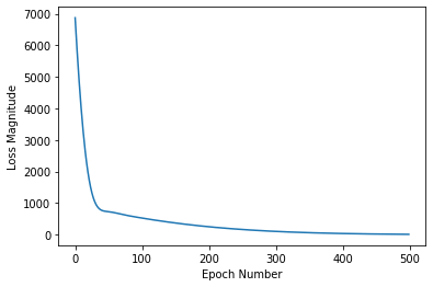
The fit method returns a history object. We can use this object to plot how the loss of our model goes down after each training epoch. A high loss means that the Fahrenheit degrees the model predicts are far from the corresponding value in fahrenheit_a.
import matplotlib.pyplot as plt
plt.xlabel('Epoch Number')
plt.ylabel("Loss Magnitude")
plt.plot(history.history['loss'])
Output
Use the model to predict values
Now you have a model that has been trained to learn the relationship between celsius_q and fahrenheit_a. You can use the predict method to have it calculate the Fahrenheit degrees for a previously unknown Celsius degrees.
So, for example, if the Celsius value is 100, what do you think the Fahrenheit result will be? Take a guess before you run this code.
print(model.predict([100.0]))
Output
[[211.28633]]
The correct answer is 100×1.8+32=212, so our model is doing really well.
Recap
- We created a model with a Dense layer
- We trained it with 3500 examples (7 pairs, over 500 epochs).
Our model tuned the variables (weights) in the Dense layer until it was able to return the correct Fahrenheit value for any Celsius value. (Remember, 100 Celsius was not part of our training data.)
Little Experiment
Just for fun, what if we created more Dense layers with different units, which therefore also has more variables?
l0 = tf.keras.layers.Dense(units=4, input_shape=[1])
l1 = tf.keras.layers.Dense(units=4)
l2 = tf.keras.layers.Dense(units=1)
model = tf.keras.Sequential([l0, l1, l2])
model.compile(loss='mean_squared_error', optimizer=tf.keras.optimizers.Adam(0.1))
model.fit(celsius_q, fahrenheit_a, epochs=500, verbose=False)
print("Finished training the model")
print(model.predict([100.0]))
print("Model predicts that 100 degrees Celsius is: {} degrees Fahrenheit".format(model.predict([100.0])))
print("These are the l0 variables: {}".format(l0.get_weights()))
print("These are the l1 variables: {}".format(l1.get_weights()))
print("These are the l2 variables: {}".format(l2.get_weights()))
Output
Finished training the model
[[211.74745]]
The model predicts that 100 degrees Celsius is: [[211.74745]] degrees Fahrenheit
These are the l0 variables: [array([[ 0.57481194, -0.31282264, -0.08991212,  0.05583713]],
      dtype=float32), array([ 3.1298614, -3.0553856,  2.024639 , -1.9173275], dtype=float32)]
These are the l1 variables: [array([[-0.11459085,  0.5284759 , -0.7752181 ,  0.09853069],
       [ 0.53424186, -1.0309159 ,  0.33990914, -0.8869713 ],
       [-0.35792652,  0.08609635,  0.42886123,  0.5282372 ],
       [-0.16600738, -0.33623806, -0.46339443, -0.4867097 ]],
      dtype=float32), array([-2.4918113,  3.0744421, -2.8050053,  3.043983 ], dtype=float32)]
These are the l2 variables: [array([[-0.60743487],
       [ 1.2982881 ],
       [-0.89300174],
       [ 1.3154573 ]], dtype=float32), array([3.0515397], dtype=float32)]
As you can see, this model is also able to predict the corresponding Fahrenheit value really well.
This is enough to digest for today, will see you next series of this article.