In the previous article on the TensorFlow series, we have read about Recurrent Neural Network(RNN) with some examples. If you haven't read here the link ->

In this tutorial, we are going to cover:

1. What is Perceptron?
2. History of Perceptron
3. Types of Perceptron
4. Implementation using Tensorflow
5. Perceptron Learning Rule

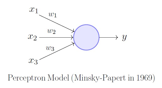
What is Perceptron?

A neural network is an interconnected system of perceptrons, so it is safe to say perceptrons are the foundation of any neural network.

Perceptrons can be viewed as building blocks in a single layer in a neural network, made up of four different parts:

• Input Values
• Weights and Bias
• Net Sum
• Activation Function

A neural network, which is made up of perceptrons, can be perceived as a complex logical statement (neural network) made up of very simple logical statements (perceptrons); of “AND” and “OR” statements.

A statement can only be true or false, but never both at the same time. The goal of a perceptron is to determine from the input whether the feature it is recognizing is true, in other words, whether the output is going to be a 0 or 1.

History of Perceptron

Perceptron was introduced by Frank Rosenblatt in 1957. He proposed a Perceptron learning rule based on the original MCP neuron.

A Perceptron is an algorithm for the supervised learning of binary classifiers. This algorithm enables neurons to learn and processes elements in the training set one at a time.

Types of Perceptron

Basically, there are two types of Perceptrons:

1. Single Layer Perceptron
2. Multi-Layer Perceptron

Artificial Neural Network(ANN)

For understanding single-layer perceptron, it is important to understand Artificial Neural Networks (ANN).

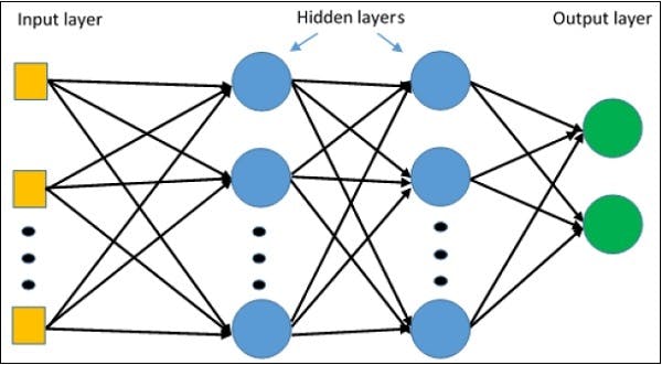
Artificial neural networks are the information processing system the mechanism of which is inspired by the functionality of biological neural circuits. An artificial neural network possesses many processing units connected to each other. Following is the schematic representation of artificial neural network −

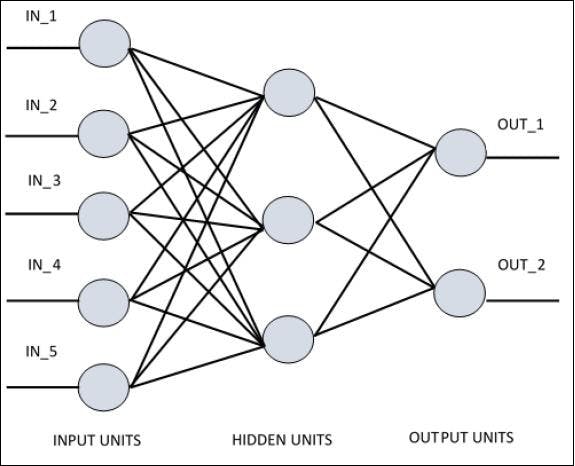
The diagram shows that the hidden units communicate with the external layer. While the input and output units communicate only through the hidden layer of the network.

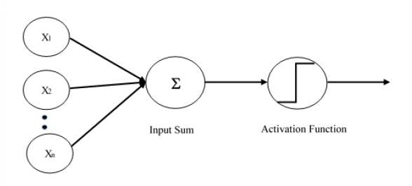
Single Layer Perceptron

Single-layer Perceptrons can learn only linearly separable patterns. The computation of a single layer perceptron is performed over the calculation of the sum of the input vector each with the value multiplied by the corresponding element of the vector of the weights.

Let us focus on the implementation of single-layer perceptron for an image classification problem using TensorFlow.

Now, let us consider the following basic steps of training logistic regression −

• The weights are initialized with random values at the beginning of the training.
• For each element of the training set, the error is calculated with the difference between the desired output and the actual output. The error calculated is used to adjust the weights.
• The process is repeated until the error made on the entire training set is not less than the specified threshold, until the maximum number of iterations is reached.

The complete code for evaluation of logistic regression is mentioned below −

# Data is used in the form of array instead of MNIST
import tensorflow.compat.v1 as tf
import numpy as np
import matplotlib.pyplot as plt
tf.disable_v2_behavior()

learning_rate = 0.0008
training_epochs = 2000
display_step = 50
# taking input as array from numpy package and converting it into tensor
inputX = np.array([[  2,   3],
                  [  1,   3]])
inputY = np.array([[  2,   3],
                  [  1,   3]])
x = tf.placeholder(tf.float32, [None, 2])
y_ = tf.placeholder(tf.float32, [None, 2])

W = tf.Variable([[0.0,0.0],[0.0,0.0]])
b = tf.Variable([0.0,0.0])

layer1 = tf.add(tf.matmul(x, W), b)
y = tf.nn.softmax(layer1)

cost = tf.reduce_sum(tf.pow(y_-y,2))

optimizer =tf.train.GradientDescentOptimizer(learning_rate=learning_rate).minimize(cost)

init = tf.global_variables_initializer()
sess = tf.Session()
sess.run(init)

avg_set = []
epoch_set = []

for i in range(training_epochs):
   sess.run(optimizer, feed_dict = {x: inputX, y_:inputY})

   #log training
   if i % display_step == 0:
       cc = sess.run(cost, feed_dict = {x: inputX, y_:inputY})
       #check what it thinks when you give it the input data
       print(sess.run(y, feed_dict = {x:inputX}))


       print("Training step:", '%04d' % (i), "cost=", "{:.9f}".format(cc))
       avg_set.append(cc)
       epoch_set.append(i + 1)

print("Optimization Finished!")
training_cost = sess.run(cost, feed_dict = {x: inputX, y_: inputY})
print("Training cost = ", training_cost, "\nW=", sess.run(W),
      "\nb=", sess.run(b))
plt.plot(epoch_set,avg_set,'o',label = 'SLP Training phase')
plt.ylabel('cost')
plt.xlabel('epochs')
plt.legend()
plt.show()

Output

Training step: 1850 cost= 13.029353142
[[0.00913966 0.99086034]
 [0.01402235 0.98597765]]
Training step: 1900 cost= 13.028603554
[[0.00889556 0.9911045 ]
 [0.0136806  0.9863194 ]]
Training step: 1950 cost= 13.027893066

Optimization Finished!

Training cost =  13.02723 
W= [[-0.21873142  0.21873151]
 [-0.57966876  0.5796688 ]] 
b= [-0.19322273  0.1932229 ]

The Perceptron algorithm learns the weights for the input signals in order to draw a linear decision boundary.

Multi-Layer Perceptron

Multilayer Perceptrons or feedforward neural networks with two or more layers have a greater processing power.

The diagrammatic representation of multi-layer perceptron learning is as shown below −

Note: Supervised Learning is a type of Machine Learning used to learn models from labeled training data. It enables output prediction for future or unseen data.

Let's build a multi-layer perceptron using Tensorflow and successfully train it to recognize digits in the image.

Let's start by importing our data. As Keras, a high-level deep learning library already has MNIST as part of their default data we are just going to import the dataset from there and split it into train and test sets.

Source code of this training here ->

1. Loading MNIST dataset from Keras

import keras
from sklearn.preprocessing import LabelBinarizer
import matplotlib.pyplot as plt
%matplotlib inline

def load_dataset(flatten=False):
    (X_train, y_train), (X_test, y_test) = keras.datasets.mnist.load_data()

    # normalize x
    X_train = X_train.astype(float) / 255.
    X_test = X_test.astype(float) / 255.

    # we reserve the last 10000 training examples for validation
    X_train, X_val = X_train[:-10000], X_train[-10000:]
    y_train, y_val = y_train[:-10000], y_train[-10000:]

    if flatten:
        X_train = X_train.reshape([X_train.shape[0], -1])
        X_val = X_val.reshape([X_val.shape[0], -1])
        X_test = X_test.reshape([X_test.shape[0], -1])

    return X_train, y_train, X_val, y_val, X_test, y_test

X_train, y_train, X_val, y_val, X_test, y_test = load_dataset()
## Printing dimensions
print(X_train.shape, y_train.shape)
## Visualizing the first digit
plt.imshow(X_train[0], cmap="Greys");

(50000, 28, 28) (50000,)

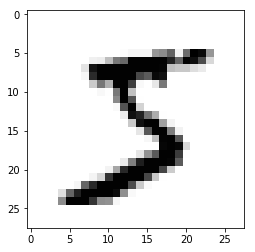
As we can see our current data have a dimension of (28 28) we will start by flattening the image in N*784, and one-hot encode our target variable.

2. Changing dimension of the input image from N2828 to *784

X_train = X_train.reshape((X_train.shape[0],X_train.shape[1]*X_train.shape[2]))
X_test = X_test.reshape((X_test.shape[0],X_test.shape[1]*X_test.shape[2]))

print('Train dimension:');print(X_train.shape)
print('Test dimension:');print(X_test.shape)

## Changing labels to one-hot encoded vector
lb = LabelBinarizer()
y_train = lb.fit_transform(y_train)
y_test = lb.transform(y_test)

print('Train labels dimension:');
print(y_train.shape)
print('Test labels dimension:');
print(y_test.shape)

Train dimension: (50000, 784) Test dimension: (10000, 784) Train labels dimension: (50000, 10) Test labels dimension: (10000, 10)

Now we have processed the data, let's start building our multi-layer perceptron using TensorFlow. We will begin by importing the required libraries.

3. Importing required Libraries

import numpy as np
import tensorflow as tf
from sklearn.metrics import roc_auc_score, accuracy_score
s = tf.InteractiveSession()

tf.InteractiveSession() is a way to run the TensorFlow model directly without instantiating a graph whenever we want to run a model.

4. Defining Various initialization parameters

num_classes = y_train.shape[1]
num_features = X_train.shape[1]
num_output = y_train.shape[1]
num_layers_0 = 512
num_layers_1 = 256
starter_learning_rate = 0.001
regularizer_rate = 0.1

5. Placeholders for the input data

In TensorFlow, we define a placeholder for our input variables and output variables and any variables we want to keep track of.

input_X = tf.placeholder('float32',shape =(None,num_features),name="input_X")
input_y = tf.placeholder('float32',shape = (None,num_classes),name='input_Y')
## for dropout layer
keep_prob = tf.placeholder(tf.float32)

6. Weights initialized by random normal function

As dense layers require weights and biases and they need to be initialized with a random normal distribution with zero mean and small variance (1/square root of the number of features).

weights_0 = tf.Variable(tf.random_normal([num_features,num_layers_0], stddev=(1/tf.sqrt(float(num_features)))))
bias_0 = tf.Variable(tf.random_normal([num_layers_0]))

weights_1 = tf.Variable(tf.random_normal([num_layers_0,num_layers_1], stddev=(1/tf.sqrt(float(num_layers_0)))))
bias_1 = tf.Variable(tf.random_normal([num_layers_1]))

weights_2 = tf.Variable(tf.random_normal([num_layers_1,num_output], stddev=(1/tf.sqrt(float(num_layers_1)))))
bias_2 = tf.Variable(tf.random_normal([num_output]))

7. Weights and Biases

Now we will start writing the graph calculation to develop our 784(Input)-512(Hidden layer 1)-256(Hidden layer 2)-10(Output) model.

We need to add an activation we will use ReLU activation for hidden layers and softmax for the final output layer to get the class probability score.

hidden_output_0 = tf.nn.relu(tf.matmul(input_X,weights_0)+bias_0)
hidden_output_0_0 = tf.nn.dropout(hidden_output_0, keep_prob)

hidden_output_1 = tf.nn.relu(tf.matmul(hidden_output_0_0,weights_1)+bias_1)
hidden_output_1_1 = tf.nn.dropout(hidden_output_1, keep_prob)

predicted_y = tf.sigmoid(tf.matmul(hidden_output_1_1,weights_2) + bias_2)

8. Define a loss function

Now we need to define a loss function to optimize our weights and biases, and we will use softmax cross-entropy with logits for the predicted and correct label.

loss = tf.reduce_mean(tf.nn.softmax_cross_entropy_with_logits_v2(logits=predicted_y,labels=input_y)) \
        + regularizer_rate*(tf.reduce_sum(tf.square(bias_0)) + tf.reduce_sum(tf.square(bias_1)))

9. Variable learning rate

Now we need to define an optimizer and learning rate for our network to optimize weights and biases on our given loss function.

learning_rate = tf.train.exponential_decay(starter_learning_rate, 0, 5, 0.85, staircase=True)

## Adam optimzer for finding the right weight
optimizer = tf.train.AdamOptimizer(learning_rate).minimize(loss,var_list=[weights_0,weights_1,weights_2,
                                                                         bias_0,bias_1,bias_2])

10. Metrics Definition

We are done with our model construction. Let's define the accuracy metric to evaluate our model performance as the loss function is non-intuitive.

correct_prediction = tf.equal(tf.argmax(y_train,1), tf.argmax(predicted_y,1))
accuracy = tf.reduce_mean(tf.cast(correct_prediction, tf.float32))

11. Training Parameters

We will now start training our network on train data and evaluate our network on the test dataset simultaneously. We will be using batch optimization with size 128 and train it for 14 epochs to get 98%+ accuracy.

batch_size = 128
epochs=14
dropout_prob = 0.6

training_accuracy = []
training_loss = []
testing_accuracy = []

s.run(tf.global_variables_initializer())
for epoch in range(epochs):    
    arr = np.arange(X_train.shape[0])
    np.random.shuffle(arr)
    for index in range(0,X_train.shape[0],batch_size):
        s.run(optimizer, {input_X: X_train[arr[index:index+batch_size]],
                          input_y: y_train[arr[index:index+batch_size]],
                        keep_prob:dropout_prob})
    training_accuracy.append(s.run(accuracy, feed_dict= {input_X:X_train, 
                                                         input_y: y_train,keep_prob:1}))
    training_loss.append(s.run(loss, {input_X: X_train, 
                                      input_y: y_train,keep_prob:1}))

    ## Evaluation of model
    testing_accuracy.append(accuracy_score(y_test.argmax(1), 
                            s.run(predicted_y, {input_X: X_test,keep_prob:1}).argmax(1)))
    print("Epoch:{0}, Train loss: {1:.2f} Train acc: {2:.3f}, Test acc:{3:.3f}".format(epoch,
                                                                    training_loss[epoch],
                                                                    training_accuracy[epoch],
                                                                   testing_accuracy[epoch]))

Training Logs

Epoch:0, Train loss: 40.71 Train acc: 0.936, Test acc:0.935
Epoch:1, Train loss: 22.14 Train acc: 0.956, Test acc:0.954
Epoch:2, Train loss: 12.20 Train acc: 0.966, Test acc:0.963
Epoch:3, Train loss: 6.90 Train acc: 0.973, Test acc:0.968
Epoch:4, Train loss: 4.12 Train acc: 0.977, Test acc:0.970
Epoch:5, Train loss: 2.71 Train acc: 0.981, Test acc:0.973
Epoch:6, Train loss: 2.02 Train acc: 0.982, Test acc:0.975
Epoch:7, Train loss: 1.70 Train acc: 0.985, Test acc:0.975
Epoch:8, Train loss: 1.56 Train acc: 0.985, Test acc:0.976
Epoch:9, Train loss: 1.50 Train acc: 0.987, Test acc:0.979
Epoch:10, Train loss: 1.48 Train acc: 0.989, Test acc:0.978
Epoch:11, Train loss: 1.47 Train acc: 0.988, Test acc:0.976
Epoch:12, Train loss: 1.47 Train acc: 0.989, Test acc:0.980
Epoch:13, Train loss: 1.47 Train acc: 0.990, Test acc:0.980

Let's visualization train and test accuracy as a function of the number of epochs.

iterations = list(range(epochs))
plt.plot(iterations, training_accuracy, label='Train')
plt.plot(iterations, testing_accuracy, label='Test')
plt.ylabel('Accuracy')
plt.xlabel('iterations')
plt.show()
print("Train Accuracy: {0:.2f}".format(training_accuracy[-1]))
print("Test Accuracy:{0:.2f}".format(testing_accuracy[-1]))

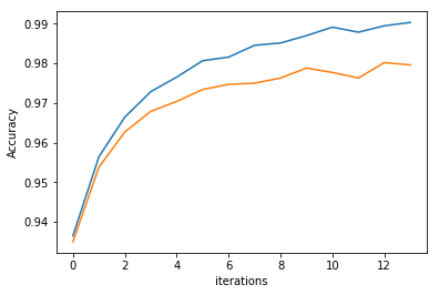
Train Accuracy: 0.99
Test Accuracy:0.98

Perceptron Learning Rule

Perceptron Learning Rule states that the algorithm would automatically learn the optimal weight coefficients. The input features are then multiplied with these weights to determine if a neuron fires or not.

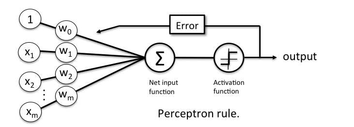
The Perceptron receives multiple input signals, and if the sum of the input signals exceeds a certain threshold, it either outputs a signal or does not return an output. In the context of supervised learning and classification, this can then be used to predict the class of a sample.

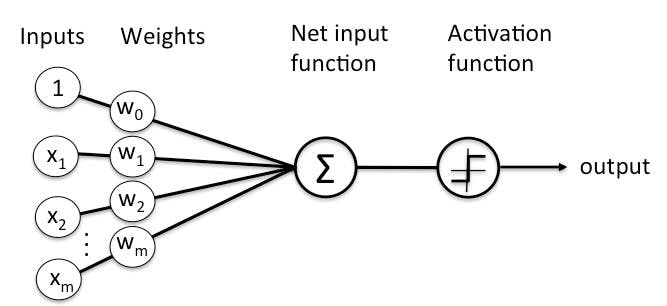
Perceptron Function

Perceptron is a function that maps its input “x,” which is multiplied with the learned weight coefficient; an output value ”f(x)” is generated.

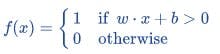
“w” = vector of real-valued weights

“b” = bias (an element that adjusts the boundary away from the origin without any dependence on the input value)

“x” = vector of input x values

“m” = number of inputs to the Perceptron

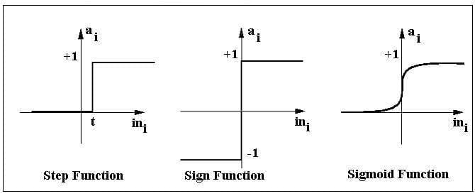
Activation functions of Perceptron

The activation function applies a step rule (convert the numerical output into +1 or -1) to check if the output of the weighting function is greater than zero or not.

For Example:

If ∑ wixi> 0 => then final output “o” = 1 (issue bank loan)

Else, final output “o” = -1 (deny bank loan)

You can read further here:

1. Perception, Importance, Factors